8 Mouse EEG Tutorial
In this tutorial, we will guide you on how to use SignalFlowEEG analyze EEG tracings from mouse multielectrode array (MEA).
Specifically, we will analzying data from the Neuronexus Mouse EEG v2 H32 probe is a 32-channel EEG MEA specifically designed for mice. Combined with the Omnetics Amplifier Adapter, it provides a complete system for acquiring high-fidelity EEG data from the mouse brain.
8.1 Overview
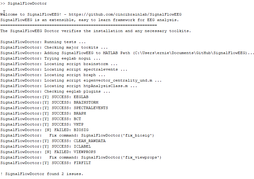
This tutorial assumes that you have already installed SignalFlowEEG (Chapter 1) and are familiar with the SignalFlow interface (Chapter 4).
During this tutorial we will calculate spectral power and run a connectivity analysis.
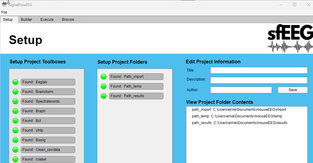
8.2 Loading Data
Create a new project folder in your filesystem to store the data and analysis results. For example,
~/Documents/mouseEEG.Create three subfolders in the project folder: ‘import’, ‘temp’, and ‘results’.
On the SignalFlow GUI select the ‘Setup’ tab and setup your project folders by assigning them to each of the three folders you just created.
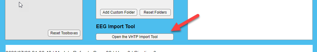
- Let’s import our mouse EEG files. In this example, we will be assuming you have already preprocessed the data into SET format. We will use the import tool to copy over the SET files to our project folder.
Select “Open the VHTP Import Tool” button underneath the Setup Project Folders pane:
- The vHTP import tool is a multipurpose utility to import data from a variety of formats into EEGLAB SET format. It also can copy SET files directly. The Import tool has the ability to select SET files across subfolders and perform keyword filtering which has advantages compared to a manual file copy.
Please refer to the vHTP import tool documentation and follow the instructions for copy SET files to your project folder (Example Workflow 2).
Link to vHTP import tool documentation
Here is example of the import tool with the SET files selected and the destination folder set to the ‘import’ folder in your project folder:
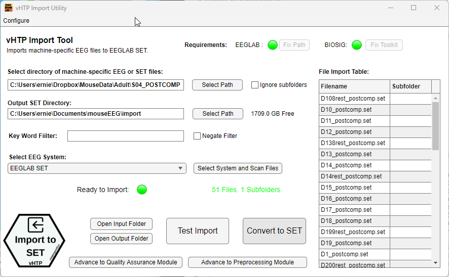
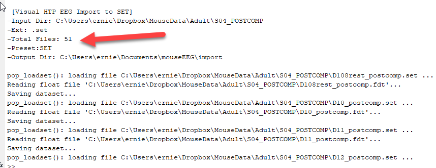
After you have selected the SET files and the destination folder, click the ‘Import to SET’ button to copy the files over. You will notice in the terminal window that each file will be loaded into EEGLAB and a channel montage graphic will be exported to confirm channel locations.
Details regarding the import will be in the command window:
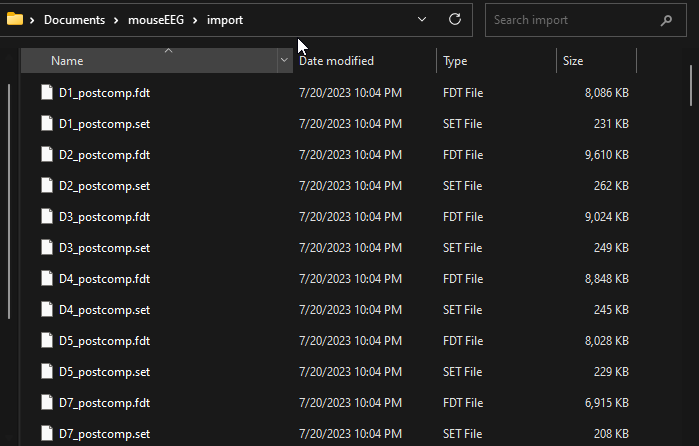
Following the import, you should see the SET files in the ‘import’ folder:
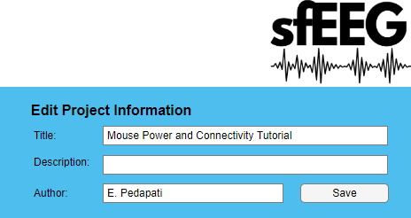
- Return to the SignalFlow Application and fill in any Project Details you would like to include. These details will be included in the analysis report.
Next move to the Builder tab to start our analysis workflow.
From the inflow modules select “Import SET” From the outflow modules select “Calculate Rest Power”
Confirm the module outflow path where the power results will be saved. In this example, we will save the results to the ‘results’ folder in our project folder.
Switch to the Execute Tab and click the “Execute (Loop)” Button to import each SET file sequentially and calculate the power. The results will be stored in table format in the ‘results’ folder.
8.3 Optional: Customize Power Bands
Published mouse EEG bands differ in exact frequencies from human EEG bands. You can customize the power bands by making a copy of the ‘Calculate Rest Power’ module and editing the ‘Power Bands’ parameter.
To start, go back to the setup tab. In your file system, create a new results folder called “results_custombands” to distinguish it from your other results folder.
Next, in the Setup tab select “Add Custom Folder” and select the “results_custombands” folder you just created. Add a easy to remember tag so you can identify it later.
Switch to the Builder tab. Click on “Calculate Rest Power” and press the “Delete Module” Button. This will remove the default power module.
Find “Calculate Rest Power” in the outflow modules and click on “Copy and Edit Module”. This will create a copy of the power module that you can edit.
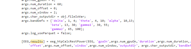
The MATLAB editor will open up with a copy of the power module. Here the parameters can be clearly seen, including the power band definitions.
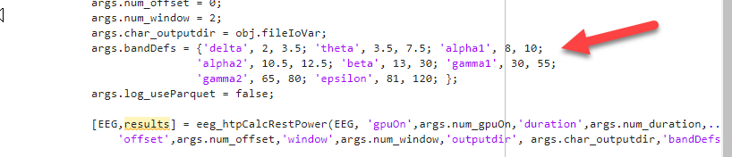
- Let’s edit the power band definitions based on Jonak et al. 2020: “Power was then further binned into standard frequency bands: Delta (1–4 Hz), Theta (4–10 Hz), Alpha (10–13 Hz), Beta (13–30 Hz), and Gamma was divided into “Low Gamma” (30–55 Hz), and “High Gamma” (65–100 Hz).”
Save and close the editor and return to the SignalFlow application.
- Let’s activate our new power module with custom bands. There are several steps to do this.
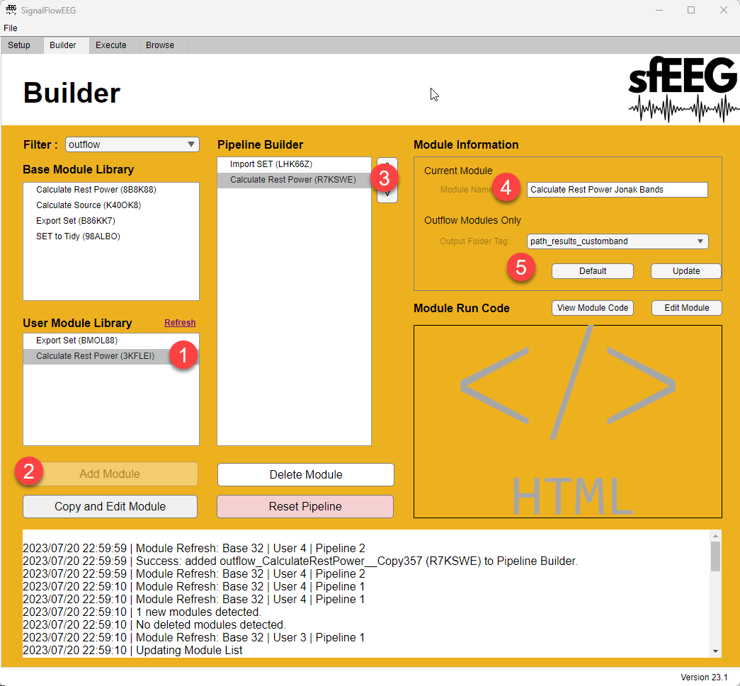
Step 1. Click on Refresh to user modules. This will load the new custom power module.
Step 2. Next, select the new module and add it to the pipeline builder by clicking on Add Module.
Step 3. Select the new power module so we can add a custom name.
Step 4. Add a custom name to the module that is more descriptive.
Step 5. Select the new output folder for the power results and select “Update”.
- Now return to the builder tab and click on the “Execute (Loop)” button to run the analysis. The results will be stored in the ‘results_custombands’ folder.
8.4 Calculating Connectivity
The vHTP function eeg_htpGraphPhaseBcm (Brain connectivity matrix) is a comprehensive function that conducts phase-based connectivity analysis on an EEG dataset. It calculates several common phase-based connectivity measures like DWPLI, IPSC, etc between all pairs of EEG channels.
It takes the input EEG data, which is expected to be epoched into trials. It loops through all channel pairs, extracts the signal for those pairs, and calculates the connectivity measures over a range of frequencies.
The output is the connectivity matrices for each measure and frequency, as well as graph theory measures calculated on the connectivity matrices.
Let’s run a custom version of this connectivity function to calculate only gamma connectivity and perform the operation on parallel processing to speed it up.
You can start right at the builder tab. Remove the power module but keep the import SET module.
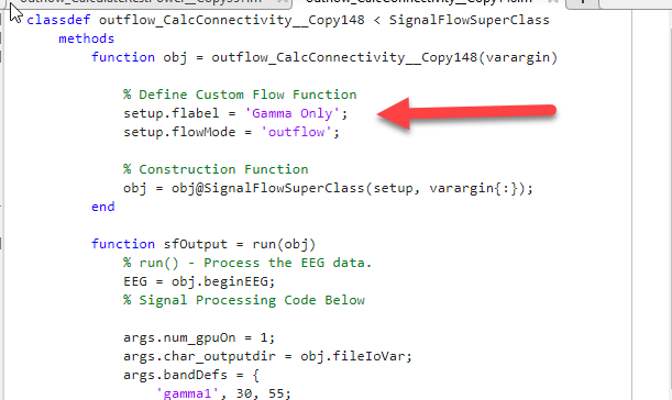
Find the “Calculate Connectivity” module and click on “Copy and Edit Module”. This will create a copy of the connectivity module that you can edit.
Adjust the bands to only include gamma bands. If you do not have a GPU, change the gpuOn parameter to 0. If you do have a GPU, you can leave it at 1.
This time we will also edit the fname to change the module name in list boxes. This is optional but can be helpful to distinguish between different connectivity modules.
Save and close the editor and return to the SignalFlow application.
At this point, you could update the description and pick an alternative results folder. Make sure to press “Update” to save your changes.
Now return to the execute tab and click on the “Execute (Parallel)” button to run the analysis. The results will be stored in the ‘results’ folder.
8.5 Summary:
In this tutorial, we have shown how to use SignalFlowEEG to analyze mouse EEG data. We have shown how to import SET files, calculate spectral power, and calculate connectivity.
The raw data files containing the values of the results can be opened across most statistical software including MATLAB.
We will next work on loading and visualizing this data in R.